Arsenal

When you are able to process an NMR spectrum; when you are also able to simulate the same spectrum (starting from the definition of a spin system); then you are ready to fit the two, one against the other. People tend to skip all the intermediate stages. I would not. If I can't write the single words, I won't be able to write a sentence. Yesterday I said that the simulation of a spin system is a useful exercise to understand a few principles of NMR; now I need to stress that it's also a useful exercise before you move on to the extraction of the NMR parameters by simulation. Once you have the two main ingredients, the experimental spectrum and the synthetic one, there are three main methods to perform the fit; each one has a reason to exist.

(1) Manual Adjustment
This can work if the spectrum, or portions of it, can be interpreted with first-order rules. Chemical shifts are easy to fit manually, because it's enough to literally drag each multiplet in place. The coupling constants can be adjusted in order, from the most evident (large) one to the most difficult (small) to extract. The process is simplified when the experimental multiplets are well resolved; in other words: apply a Lorentz-to-Gauss resolution enhancement by weighting the FID. Manual adjustment has become quite popular after the advent of interactive applications in the 90s. Don't dismiss it as "naive": it is certainly more accurate than extracting the coupling constants directly from the list of frequencies (which is an accepted and widespread practice). Visual fitting can be difficult with second-order spectra, but not for a skilled operator. The trick of the experts is to monitor the position of the weak combination lines. They are forbidden transitions that appear as tiny satellites. If you can simulate them exactly, the rest comes naturally in place. They are diagnostic, like canaries in a coal mine.

(2) Laocoon
This was the name of the first popular program used to extract the Js from second-order, complicated multiplets. The program is no more in use today, but the method is still excellent. Quite simply it compares a list of experimental frequencies with a list of theoretical lines. Then improves the spectroscopic parameters according to the least squares principle. A lot of useful information is ignored, but this is also the strength of the method. When there is too much noise, or the baseline is problematic, or a solvent hides part of the spectrum, etc... you simply can't extract all the information from the spectrum, or you can but the intensities are not dependable. It's better to feed the algorithm with minimal selected data of high quality than hoping that a mass of errors can mutually compensate each other. With Laocoon it's not even necessary to match all the lines; as you can expect, the condition is that the number of parameters to guess must be less than the number of the lines. Despite the simplicity, this method requires more work, because you have to assign/match each experimental line to a theoretical line. This job looks trivial at the end of the process, because it's enough to match the lines in order of frequency. It's different when the starting guess is largely inaccurate. A single mismatch, in this case, is simple to discover, if you know the trick. The column of the residual errors will contain two large and opposite values. They correspond to the "swapped" lines. All considered, the most difficult part, for the user, is to read the manual of his/her program.
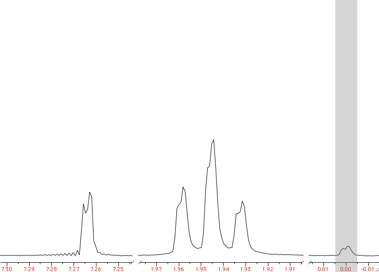
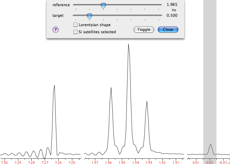
Here, more than in any other case, a Lorentz-to-Gauss weighting is beneficial: remember that you are not starting from the raw data points, but from the table of frequencies ("peak-picking"). It is well known that the position of the maxima of a doublet doesn't coincide with the true line frequencies, when peaks are broad.

picture courtesy of the nmr-analysis blog.

(3) Total Line-shape (TLS)
I suspect that this approach derives, historically, from dynamic NMR, (the simulation of internal rotations, like in the case of DMF). You can, indeed, simulate a "static" system with a dynamic program, if the exchange rate is zero. DNMR (and the programs that follow the same principle) don't recalculate the single lines (frequencies, intensities) but other sets of parameters that are used, eventually, to create the synthetic spectrum (plot). The latter can be compared, point by point, to the experiment, and the least squares are calculated from the difference. This is a great simplification for the user, compared to LAOCOON, because it's no more necessary to assign the lines. An higher quality of the experimental spectrum is however required, because the program now also employs the intensity information, and this information must be correct. Therefore the baseline must be flat and no extraneous peak can be present (it is trivial, however, to artificially delete isolated extraneous peaks/humps). Summarizing: you must spend time on processing the experimental spectrum.
We have seen that the first two methods prefer gaussian line-shapes.
This is not necessary with TLS, but we have the inverse problem: if you have already prepared the experimental spectrum for the other kinds of fit (with Gaussian shapes), can you perform a total lineshape fit? The answer is "NO" if we look at the original formulation of the method, but in practice it is possible, with some commercial package, to work with both kinds of shapes (and anything in between too).
Don't be mislead by the name "Total": nobody fits the whole spectrum, but only portions of it. Most of the tricks we learned when fitting singlets (and collection of not-organized peaks) can be recycled with TLS. Actually, there is a minimal difference, from a mathematical point of view. In TLS, the algorithm varies a collection of parameters. They give a collection of lines, that are used to simulate the spectrum. In deconvolution, the algorithm directly start from the frequencies. That's the first difference. There is also a procedural difference: TLS has a built-in mechanism to escape from local minima. In practice, in the first stage of the fitting, a line broadening is applied that blurs the details. Once the multiplets has been set in the proper place, the broadening is removed and the details are taken into account. With plain line-fitting, there is no such need, because the first guess is extracted from the experimental spectrum itself, therefore everything is always in the right place (nearly).
If we called the previous method by the name of the first program implementing it, then TLS could be called, in a similar way, "DAVINS".

Spin Systems

A fortnight ago we saw how to fit a spectrum with a collection of curves. A more evolute approach is to fit the spectrum with a collection of NMR parameters (shifts and Js in the first place). There are two reasons to prefer the latter approach:

1. you introduce logical restrictions into the model, for example you specify that the components of a triplet are in the ratio 1:2:1
2. you overcome the job of measuring shifts and Js from line positions

Simple line fitting to a generic collection of lines remains the best choice for singlets, simple multiplets and when you are not interested at all into the frequencies, but only into the intensities. Simplifying, curve-fitting (the so-called "deconvolution") is more about areas, spin system analysis is more about energies.
We have arrived to a large topic from an unusual path. We are in the field of quantum mechanic. It's easy in theory and, in practice, when the nuclei are few. When the number of nuclei in a spin system grows, no computer is fast enough to calculate precisely what happens. Somebody has also proposed to invert the roles, and create a super-computer with a large enough spin system (the quantum computer). That's even more difficult (try building a real molecule with 20 different nuclides!). When the number of nuclei is limited (e.g.: 10 protons), there is however no problem, at least with the older programs that diagonalize the Hamiltonian. I dedicated a post to the modern programs that can follow the evolution of a system under all kinds of effects. They have more calculations to do, are limited to smaller systems and, as it appeared from my old post, are oriented towards solid-state NMR.
Older programs are more popular in liquid-state NMR. I have already cited the free gNMR and SpiWorks. I have probably never cited Perch LE and Wind-NMR. Thay are all free (for academic users at least) and they all require Windows. Can you suggest a free solution for Linux and Mac users?
It's not a surprise that, which such an abundance of free solutions, the commercial applications, in this present moment, are ignoring the field. The race now is at predicting the spectrum directly from the chemical structure. That's the third level. At the first level we have the frequencies and intensities of the single lines. At the second level we have shifts and couplings. At the third level we have the structure. If you only have the third level, you can verify your spectrum against the prediction, but if you want to publish your data you need to extract the Js directly from the experimental data. You can't do that without the second level, unless you are glad to standardize all your reports into lists of unspecified multiplets, like:
7.24, m (2H); 4.14, m (2H), 2.36, m (8H).....
The simulation of spin systems is also becoming a popular exercise for chemistry students new to the world of NMR. It's amazing how fast the magnetic field can change, even by orders of magnitude. After a while the game becomes repetitive, but it remains highly instructive for newcomers. An excellent starting point is an article by Carlos on the NMR Analysis Blog. It should be, however, complemented by practice, more than by further references. There is a minimal library of ready examples for Mac users. It contains the classic cases (orto-di-chloro-benzene, DMF), plus templates for small and medium-sized systems of 1/2 nuclei. In the case of DMF you can change not only the magnetic field, but also the temperature.
I don't want to bother you with theory, but one thing at least must be said: geminal couplings usually have a negative constant!
One more thing on practice too: Carlos said that not all NMR signals are symmetric. Personally I still believe into the myth that they are symmetric, like the human body. To be precise, neither are symmetric, but in practice this precision is useless and misleading. I rely on the IDEA of symmetry to recognize a friendly face and I rely on the IDEA of symmetry to recognize NMR signals. By the way: they too are friendly!

Fixed Focus

All cameras need to be focused before shooting. There are 3 alternatives: manual focus, autofocus and fixed focus. The latter is an economical choice that can't work under all circumstances, it's OK only when the depth of field is large enough. This depth depends on the characteristics of the lens.
I can see a similarity in NMR spectroscopy. The phase correction of an high-resolution spectrum is like a lens with a limited depth of field (think to a telescope, if you are more familiar with them; the telescope is an example of a lens with a narrow depth of field). Starting from the optimal correction, a minimal change in the phase correction parameter (movement of the lens, in the parallel example) causes a visible negative effect on the spectrum (clearness of the image). It's not enough to copy the phase correction from a spectrum to the other, you must use either manual or automatic correction or both. Like it or not, you'll become an expert in the field.
Weighting is much more tolerant to a small change of the parameters, to the point that most of us use the "Fixed Focus" approach. We can even store the optimal value inside our standard parameters and forget about it. When you have forgotten it, it's arduous to improve your skill; DSP (digital signal processing) contains too much theory and practice is time consuming.
My rules are:

1. Weighting is an alteration of the spectrum. An altered spectrum may look ugly, don't worry.
2. It's more important to know what I want to obtain (where I want to go) that the way to go there, because many roads lead to the same place, but I must be able to recognize my destination if I arrive there.

While I usually recommend to observe and practice, because 50% of NMR can be deducted with common sense, there is a case where you need the theory, otherwise you go nowhere. If you keep weighting a standard COSY spectrum with the same functions that you use in 1D spectroscopy, you'll always get star-shaped peaks like this:
[after exponential weighting along both dimensions]

It's only theory that tells you that a symmetric FID corresponds to a symmetric spectrum, therefore if your weighted FID has a symmetric envelope, the dispersion component will be attenuated in frequency domain. In simpler words: use a sine-bell. It's counter-intuitive to zero the less noisy part of your spectrum, but look at the final effect:
[after weighting with two pure sine bells]

Recollection

Before the touristic digression, we were slowly coming back to an old topic: Reference Deconvolution. If you are new to this blog, RD it's an alternative technique to weighting. Think at it as "tailored resolution enhancement" or "shimming-after-the-fact". I commented on it in two recent articles:

Reference Deconvolution in Theory

Reference Deconvolution in Practice

Tremiti Islands

Last Thursday I visited these islands for the first time.



Pictures by Maria Luisa.

Asterisk or pizza?

At the basis of weighting there's the convolution theorem.
FT( f ⋅ g ) ∝ FT(f) * FT(g)
which can also be written as:
FT( f ⋅ g ) ∝ FT(f) ⊗ FT(g)
The choice depends, exclusively, on which symbol you use to indicate the convolution operation. If, after reading the linked Wikipedia pages, you feel like being still at the point you had started from, I can propose a simplified approach, based upon Fourier Pairs and practical examples. If, in time domain, you have an exponential decay, after FT you get a Lorentzian curve. The two functions form a Fourier pair. The Gaussian function pairs with itself. A stationary sinusoid pairs with an infinitely narrow line (a nail pointing upwards). It's a curve with no shape and no width (but it has a frequency). Convolution of two curves yields a third curve with the shape of both ancestors and a patrimony (line-widths) equal to the sum of the widths of the ancestors. You can think at the result curve as an empty and opaque envelope with no shape, with both ancestor curves inside. The envelope adheres to the content, so you can see the cumulative shape.
The natural NMR peak can be described, in time domain, as the product of a stationary sinusoidal wave with an exponential decay. This dumped sinusoid forms a Fourier pair with the convolution of a nail with a Lorentzian curve. This is the convolution theorem (applied to NMR): multiplication in time domain is equivalent to convolution in frequency domain. If you consider the wave as the substrate and the exponential decay as the weighting function, the result takes the frequency from the former and the shape from the latter. That's OK. You can't do the contrary (positive substrate and oscillating weight). If your weighting function oscillates, all the peaks will show an extra splitting.
Let's give, now, some reference formulas. We'll use the symbols:
W = full linewidth at half height, always measured in Hz
ν = frequency (Hz)
ω = 2 π ν = angular frequency
The exponential decay, in time domain, is described by a single parameter λ:
f(t) = exp( - λ t ).
It forms a pair with the Lorentzian curve in frequency domain:
F(ω) = λ / (λ² + ω²).
The latter has linewidth:
W = λ / π.
That's the only parameter I consider, instead of λ, because W can be directly compared to natural signals or to the gaussian broadening.
The Gaussian curve, in time domain, has the formula:
g(t) = exp( - σ² t² / 2 ).
The other component of its Fourier pair is still a gaussian function:
G(ω) = √{ 2π } ⋅ exp[ -ω² / (2σ²) ] / σ.
σ = π W / √{ ln(2) } ≅ 3.77344 W.
The exponential lends itself to both kind of uses (it can increase either the sensitivity or the resolution, it's enough to invert the sign of λ). You can also define a new function:
1 / g(t) = exp( σ² t² / 2 ).
to increase the resolution. It's unmanageable: σ could only have near-to-zero values (otherwise the noise becomes intolerable); to the best of my knowledge, nobody has ever used this abort of weight.
We have arrived at dividing, instead of multiplying. If multiplication in time domain is equivalent to convolution in frequency domain, then division is equivalent to deconvolution...

If I Had a Bell

Weighting functions are so easy in practice and so (apparently) difficult in theory, that I wonder if we can just ignore the latter and pretend it doesn't exist. It's a matter of language. Instead of moving towards simplification, we keep creating more names, more languages, more ways to measure things. If you have learned NMR from the literature, you'll discover a different language in software, and can't find the vocabulary for the translation. The same happens when you want to write your own article: how you describe your NMR processing? It's the inverse translation. Last but not least, different softwares have different names and units for the weighting functions. Don't be mislead by the names, what matters is the shape of the window function. Ideally, it should be reproduced into your manual. Given that the shape often depends on a user-settable parameter, they can't illustrate all the possible cases. You can, however, ask the program to show the plot of your weighting function and/or the weighted FID. This is the best vocabulary. If the function grows (moving from left to right), then it can enhance the resolution.
Apart from this effect of visual translation, it's neither necessary nor advisable to observe the effect of the weighting function on the FID, when you can directly observe the effect on the spectrum in frequency domain. The FID is dominated by a few intense signals, often coming from the solvents, that are of little importance to you. In frequency domain you can monitor the effect of weighting on the important signals only.
Remember that weighting means selective attenuation, but also alteration and degradation, which you must be ready to accept: it's a part of the game. It improves the appearance of some signals and not of others. I go to the frequency domain, zoom into the region that I want to improve, and monitor the effect of varying the parameters (just like phase correction).
In some cases there's no parameter to adjust. Typical is the case of the squared cosine bell. It has a shape similar to that of a gaussian bell and it means that you could equivalent similar results using either. It's easy to calculate which value you need for the sigma, in case you choose the gaussian function, but it's even easier to use a cosine bell, with no parameter at all to set!
blue: weighted with a squared cosine bell
red: weighted with a gaussian bell (line broadening = 0.93324 / acquisition time).
The example contains four lessons:

1. non branded weighting functions can be better than the branded ones
2. anybody can be creative with them
3. there's no optimal weight and, even when it exists, a small variation corresponds to another weight that's almost as good, for all practical purposes.
4. If your software provides a limited number of functions, it doesn't mean that your possibilities are limited.