
Sunday, 28 December 2008
Tuesday, 25 November 2008
Wrap Up
When you split an article in pieces on a blog, they appear in reversed order, so it's not a great idea. A summary helps:
To be honest, I have not described all the details. I feel I have been pedant enough. There is another trick yet. If you select multiple items, the preview window shows additional controls. Without explaining everything, here is the picture:
To be honest, I have not described all the details. I feel I have been pedant enough. There is another trick yet. If you select multiple items, the preview window shows additional controls. Without explaining everything, here is the picture:

Tuesday, 18 November 2008
Coda
In this fourth and final part of the article, we'll discover the flexibility of the metadata system. For example, let's say you don't like the slideshow. A single picture is enough. You want, however, to inspect the metada. In the second part we learned that the command "Get Info" satisfies this need. The new command "Quick Look" can generate a different representation. It shows the same information (more or less), with an HTML layout and much larger fonts. In other words, it's more readable:

There is also the opposite way of doing things. Let's say that you want to see your list of files in text form, without icons and thumbnails, without the coverflow effect, but you want to see the preview of your files nonetheless. Here again the "Quick Look" command comes to the rescue. It opens a glassy, dark-grey window, that acts as an ispector. When you select a file, the preview window shows the internal pages. You can use the scrollbar (or the keys PageUp and PageDown) to move through the pages. If you select a different file, its contents are automatically shown.

The preview also includes an optional Full-Screen mode, when all the other windows are hidden and the background is black. You activate this mode by clicking the symbol with two white arrows. The full screen-mode is too large to be shown here.
None of things described in my article will help you to make a discovery. That's normal. Do you ask to the computer hardware to increase the number of your publications? I think not. Why, then, should we ask such a thing to the software?
Slideshow
In the second part of this article we saw the coverflow effect. In this third part we'll see what happens when we move the mouse near to one of the thumbnails.

Two arrow controls appear. They let us browse the internal pages of a document. In the case of a spectrum, the pages can correspond to some important details or to user comments. Alternatively the user may choose to change the display mode. In our example, the integrals are shown on the first page only, the peak frequencies on the second page only.

In practice, the computer has automatically generated a slideshow presentation for you. This becomes very useful indeed when you want to browse your spectra of yesteryear, or when your boss asks you how are things going and you obviously have no time to prepare a PowerPoint presentation.

If you click the above pictures you can see them at their natural size.
Metadata
It's not easy to obtain the permission to show a nice spectrum. For this article I have downloaded a collection of spectra of a standard compound from the Biological Magnetic Resonance Data Bank. They are not very nice but can serve my purpose. I have also processed the spectra to highlight the relevant information.
Now I'll show you what is visible after you close the processing application. All the snapshot are taken while working with the operative system. I have uploaded very large pictures, so you don't lose too much (you'll only lose the animation effects). The blog shows them at a reduced size, but if you click a picture, the full-size original appears.
As a starting point, I have selected a file, without opening it; the command "Get Info" shows this panel:
 This is only moderately useful, because selecting a file is already a time-consuming operation (you have to navigate through the folder hierarchy). The good news is that the computer can find the spectra for you, if you specify the same properties. This is the job of the command "Find". For example, we can ask the list of all the files relating to substances of general formula C5H7NO3:
 Yes, the computer understand a chemical formula! Such a search is not restricted to NMR documents. We can however add more conditions to restrict the search, how many conditions we like. For example:
 Every time I type a single character the list of results is updated (live). There is also the option of displaying an animated list. It's a cinematic effect that's very characteristic. If you have ever seen iTunes or the iPhone you know what I mean. On my blog I am limiting myself to displaying static pictures, however. Here is how my spectra look like:
 And this is only the appetizer! [continues...]
Monday, 17 November 2008
What's New
For more than two years I have been describing application software ("the programs"), and not the operative systems. Sounds obvious? It isn't. I had noticed, in the past, the attempt of a couple of programs (namely the ACD suite and the "NMRnotebook") to substitute the operative system. What they do is to put all your NMR data into a monolithic archive. From that moment on you can't search your files into the normal directory tree: the application program manages everything, substituting for the system. Can they do it better?
I have also seen the opposite phenomenon, that is the appearance of new operative systems that do every kind of things, up to the point to make you feeling that application programs are no more necessary. My preference goes to the latter trend, for a practical reason. When you are in troubles with an operative system, you can find a neighbor or relative that knows it well and that can help you. If you are at work, you can call the IT department. If your troubles arise from the application software, instead, you don't know whom you can turn to. That's why I prefer doing more things than possible with the operative system, if I am allowed.
While I will be describing a specific OS, I am writing for everybody: it's the idea that counts, not the implementation.
Now, in my life I have studied only two OS. The first one was called "IBM-DOS" and the second one "MS-DOS". It happened in an era when the computers included heavy and bulky printed manuals. I have been commuting for half of my life, so I had plenty of opportunities to read paper manuals (over and over again). I am not using those OS any more and I have forgotten what I had learned. I have come in touch with the modern systems, but still feel like a stranger (I haven't found the new manuals yet!). Last week I have begun working with Mac OS 10.5.5. It resembles the old version 7 that I was using in the early 90s, so it looks familiar to me. I have tried to read the installation manual, which shows a few things you can do but doesn't tell how to do them. It only explains how to install the system. I am learning by practice.
The rationale is that customers don't know what to do during the endless installation process, so they are given a manual to spend their time with. Unfortunately, you can read as slowly as you possibly can, but the installation will always be slower than you. To give you an idea, the whole manual, including the unreadable license agreement, weights 94 g.
What has this to do with NMR? Well, this OS seems to be almost ready to handle NMR data out of the box. I want to show you the technologies that I have explored so far, and they are enough to write posts for a week. Mainly I will describe two commands: "Get File Info" and "Find...", that are so ancient I believe they have always been there, with the same keyboard shortcuts (maybe under a different menu). What's new? Now you can install custom plug-ins for those commands. The operative system will instantly become NMR-savvy. Writing a plug-in is not terribly complicated. The Apple site gives you all the tools, libraries, instructions, examples and templates you need. You can write a plug-in in an afternoon. If you have more time, with the same tools you can even write a complete NMR program. No need to look around for the FFT algorithm, it's already a component of the OS. Of course, it has been put there to manipulate sounds, not to process NMR spectra. If you can't write a line of code and want everything ready and free... then you are lucky! What I will be showing during this week can be done with freely available plug-ins. You don't need to know how to write them.
Let me clarify my intent. It's not that I am supporting Apple. I think it's a greedy corporation, no better than Microsoft or IBM. Their products are over-priced in the U.S. and sold at an outrageous price elsewhere. I would rather encourage you to stick to your old hardware and software. (Beware that programs written for System 7 are not compatible with 10.5). Nonetheless, it's nice to be curious about the new technologies. What I have discovered last week sounded new to me, probably is well known to you, surely will become normal practice in the near future. Enough said, for today [continues...].
Sunday, 26 October 2008
ProSpect
A rare event: I have found an NMR program that's been a pleasure to inspect. It comes with an HTML manual (with pictures) and sample data. These two ingredients remove the usual obstacle for learning (you rarely guess right how to arrive to a frequency domain spectrum). In this case, instead, I could easily open one of the included sample spectra, because they come with their own processing scripts, and experiment with the buttons (relying on the help of the yellow tips). It's clear that they spent their time and money in making this program. It's well done.
The program is called ProSpect ND and comes from Utrecth. It's completely free. In theory, it's cross-platform. I have tested the Windows version.
Why isn't it more famous? Well, to start with the name, it is focused on multi-dimensional spectroscopy and favors serious processing and flexibility over simplicity of use. You realize this fact from the very beginning. To open a spectrum (Bruker or Varian, no other format is recognized) you must first convert it into the ProSpect format with a script; it's not trivial.
The program also includes all the routines to process and analyze a 1D spectrum. The graphical layout is, well, arguable. For example, the peak-picking labels tend to overlap with each other.
 Speaking of 1D, LAOCOON is also included. Forgive my personal reminiscence: the manual doesn't refer to the first version, as everybody else has always been doing, but to the the last version by Cassidei and Sciacovelli, who happen to be the ones who teached me how to use a spectrometer (and some theory too, in the case of Sciacovelli).
 My first impression: they have written a program the way they like it. If you need to print your 1D spectra, I bet you'll have diverging opinions. If you like to spend much time in 2D processing to obtain the optimal results, and the other free alternatives don't satisfy you, chances are that ProSpect ND will.
 This product confirms the rule: it takes time and money to make NMR software. If you want it free, you must find a sponsor with large shoulders. There's an important difference that puts ProSpect apart from more famous free programs like the original Mestre-C, NMRPipe, SpinWorks, NPK. Prospect is open source. In the case of NPK I may be wrong. Anyway, you can directly download all the source code of ProSpectND without asking any permission, without registering, without logging in. Guess the language? Phyton? Noo! Java? Noo! C++? Noo! OK, here's an hint: the first date on many source files says 1997.
C? Yes, I like it!
Friday, 24 October 2008
Students
They say that students buy Macs. Is it true? If it is so, and you are a student, be sure to check this promotion out. It's a full-fledged, up-to-date application, offered at a price that's certainly affordable for any student. It's possible to test the product before buying it, of course.
...and you can even leave your comment here below!
...and you can even leave your comment here below!
Friday, 10 October 2008
End of the World
Il mercato ormai di questo ritmo sta scontando la fine del mondo, altro che recessione! Se per caso avete perso del denaro in questi giorni, potete consolarvi in fondo era solo carta straccia. Presto torneremo al baratto, torneremo ad essere agricoltori, due galline, una capretta per il latte, ci potremo sedere intorno ad un focolare e stringerci con i nostri familiari e le persone più care, il pianeta non sarà più inquinato, sarà un luogo più vivibile,niente stress, niente lavoro forzato, il capo che rompe le palle, niente più calcio e calciatori fighette, niente più auto, Briatore e cocainomani del billionaire, niente più grande fratello e isola dei coglioni...che spettacolo forse stiamo andando verso un mondo migliore e allora forza S&P 500 ancora 900 punti verso lo zero! Hahahaha!
taken from Ferro Azzurro
Will all the NMR programs resist to this crisis?
taken from Ferro Azzurro
Will all the NMR programs resist to this crisis?
Thursday, 2 October 2008
Whitening
In 2007 Carlos proposed to me a joint project to invent a new algorithm for 2D automatic phase correction. There were two reasons why I replied negatively. First thing first, I am doing research with no grants and no salary. Although there was the certainty of making some money in case the algorithm had been invented, I was doubtful that I could invent this thing any time soon. The second reason was that I have fun correcting the phase manually and I didn't want to spoil my fun. Instead of admitting that any normal person would benefit from an automatic procedure, I am still tempted to teach manual phase correction to everybody, guessing that they can have the same fun that I have. Carlos accepted my answers, at least the first reason. The story seemed to end there, but it was not forever.
This summer I wrote to Carlos that I really couldn't find anything interesting to do during my holidays and that it was better to do some work. He said he had an idea to keep me busy. Guess what? Inventing the automatic 2D phase correction. This time I agreed. I proposed a three-steps roadmap. The first step consisted into trying to correct the phase of a single isolated peak, adjusting simultaneously the 4 parameters involved. The second step was a semi-automatic method in which the user was required to select any number of peaks, even of different sign, and the computer had to do the rest. The preliminary method invented at the first stage would have been the main ingredient. The third stage was the completely automated method.
I liked this roadmap because the first stage looked feasible (I hate wasting time on hopeless research). The other stages were challenging, but, in my heart, I was hoping to find an escape route before arriving there. I was glad enough to have something to do for the first week.
Carlos asked me if I wanted any 2D spectrum to test my ideas. He had already mentally created a list of different cases with different characteristics. An important case was the edited HSQC, containing both positive and negative peaks (and more noise; and no diagonal). It looked more difficult then the other cases. I said: "I have never acquired this kind of spectrum; send me a specimen". When the file arrived I was already working on my project, but not making any progress because my code was infested by bugs (I was out of shape). I suspended my activity to inspect the edited HSQC. Processing it was a relaxing activity, which I did on autopilot. When I saw the 2D plot in front of me, I said to myself: "What have you done? You have corrected the phase without paying the least attention to which peaks are positive and which are negative. Actually you haven't even paid the least attention to where the peaks are located, but the phase is perfectly corrected! What does it mean?"
There was an explanation. Manual phase correction is ALWAYS so easy, at least the coarse correction is easy. I know that if I am moving the slider into the good direction, peaks become narrower and take less space into the map. Because my background is usually white, I know that if the white regions are growing, that is a sign that I am going into the right direction. I stop when the white regions start shrinking again. I immediately realized that my mental process could be easily translated into a computer algorithm. I also noted that the correction along the X axis is independent from the correction along the Y axis. The four-dimensional problem could be factorized into two bi-dimensional problems, easier and faster. I suspended the original project and began to write the new algorithm. In 24 hours I verified that it worked and worked very well. I also debugged the old code (belonging to the original project) and discovered that it was quite unstable: it only worked under ideal conditions.
I was forced to abort the first project, but very happy of having invented something really useful and really new (in a single stage). The weakness of the aborted project was that it had to observe a limited number of points at each time. The whitening method, instead, looks at one million points simultaneously. It's a statistic measure and it's reliable just because it condenses one million of observations.
Today the whitening method is a component of 3 commercial products. It has been already presented at a meeting and (in the form of poster) at a conference. We have written an article and submitted it to Magnetic Resonance in Chemistry. You may be wondering what the hell we could have written into that article, if six words are enough to state the method: "maximize the number of white pixels". Wait and see. I am convinced that the article will be accepted just because the principle is clear (have you noticed the pun?). If they have published (in many cases of 1-D automatic correction) the articles that describe algorithms that nobody has never seen in practice, why shouldn't they publish ours? Our products can be freely downloaded and you too can test the algorithm!
The natural question is: if this method is so obvious and simple, why nobody else had invented it before? The answer can be found inside Carlos' blog. While I have been performing REAL 2D phase correction for years, there are people that even ignore that such a thing is possible. What they are doing is the correction of selected rows and columns (traces) or their sum. Actually it's a mono-dimensional correction, but they believe it's a 2D correction. A pertaining example can be found on Glenn's Bruker-oriented blog. I have had the privilege of performing true 2-D manual correction and it helped me.
Finally, I must confess: I am having a lot of fun with automatic phase correction and after I have invented it I don't want to go back!
Wednesday, 1 October 2008
Commuting
The canonical sequence is:
Rance -> FT -> shuffle -> FT -> shuffle -> FT
This is the result:
The following sequence also arrives there:
FT -> Rance -> shuffle -> FT -> shuffle -> FT
which proves the commutability between FT and Rance. When I try this:
FT -> shuffle -> FT -> Rance -> shuffle -> FT
the result is:
Rance -> FT -> shuffle -> FT -> shuffle -> FT
This is the result:

The following sequence also arrives there:
FT -> Rance -> shuffle -> FT -> shuffle -> FT
which proves the commutability between FT and Rance. When I try this:
FT -> shuffle -> FT -> Rance -> shuffle -> FT
the result is:

Tuesday, 30 September 2008
Ray Nance
I have a challenge for you. It's a puzzle that I can't find the solution to. Before your challenge, I need to finish the story of my challenge (I already told the beginning and the middle part: see previous posts). To tell my story, however, I need to explain my language first. When I asked for help, on September 9, nobody understood what I really needed, because we speak different languages. While I look at the mathematical description of NMR processing, you think at the software command that performs it. This time I will try to be the clearest I can. The world of NMR is complicated because every program stores data in a different way. There is the sequential storage and the storage in blocks, the little endian and the big endian, the interleaved and the non-interleaved. Add to this that the spectrometer is free, when writing the data on disc, to change the sign to a part of the points. When acquiring a multidimensional spectrum, which is made of many FIDs, it is also free to collect those FIDs in any order (this is the case of Varian's, which has two different ways to acquire a 3D spectra, although one was enough, and none of the two ways is vaguely similar to the Bruker way...). NMRPipe adds a further complication, because when it read Varian data it changes the sign (and the users can't know). There are also different FT algorithms that don't yield the same spectrum (the real part is always the same, but the sign of the imaginary part looks like an arbitrary choice).
I don't want to talk about these dull details: they are hackers' business (and, unfortunately, my business too).
I want to talk, instead, about phase-sensitive detection, because this is where my deepest troubles came from.
Phase-sensitive detection brings so many advantages, in terms of sensitivity and resolution, that it's almost a must in NMR spectroscopy. To accomplish it, the spectrometer measures the magnetization twice (in time or in space). When the spectrum arrives on the disc, two numbers are stored where there used to be one. To accomplish phase-sensitive detection in bidimensional spectroscpy, two FIDs are acquired instead of one. To accomplish phase-detection in 3-D spectroscopy, two bidimensional experiments are performed instead of one. In summary, a 3D FID contains 8 values that correspond to an identical combination of t1, t2 and t3 coordinates (a couple of couples of couples). In practice it can become a mess, but the rules are simple enough. Whatever the number of dimensions, each and every value has a counterpart (think like brother and sister). You don't need to think in terms of rows, planes or cubes. Just remember that each sister has a corresponding brother and vice versa. There is no difference between 2D and 3D spectra. There is an extra operation, however, that is absent in 1D spectroscopy. It's called the Ruben-States protocol (you can add more names to the brand, if you like; I call it, more generically: "shuffling"). How does it work?
We have a white horse and a white mare (brother and sister). We know that every mare has a brother and every horse has a sister. This is also true for the mother of the two white horses. She had a black brother, with a black son and a black daughter. Now, let's swap the black horse with the white mare. The members of the new pairs have the same sex. With this combination you can continue the race towards the frequency domain and win. The trick works in almost all kinds of homo-nuclear spectra. In the 2D case, you have to perform two FTs. The shuffling goes in between. In the 3D case, there are 3 FTs and 2 intermediate shuffles: FT, shuffle, FT, shuffle, FT. Maybe you have heard about alternatives called States-TPPI or the likes. Actually they all are exactly the same thing.
Our trick is not enough when gradient-selection is employed in hetero-nuclear spectroscopy. You hear the names "sensitivity enhanced" or "echo-antiecho" or "Rance-Key". It's easier for me to remember Ray Nance instead, although he had nothing to do with today's subject. Whatever the name, this kind of experiments require an ADDITIONAL step, to be performed before anything else, or at least before the shuffling. Here is what you have to do. Let's say that A is the pair of white horses and B the pair of black ones. Calculate:
S = A + B.
D = A - B.
Now rotate D by 90 degrees. This latter operation has no equivalent in the realm of animals. It would consists into a double transformation: the brother would become female and the sister a... negative male, if such an expression has any sense. Finally, replace A with S and B with the rotated D.
The 3 operations involved (addition, subtraction and phase rotation) all commute with the FT. Knowing this fact, I have always moved Ray Nance from his canonical place (before the first FT), to the moment of the shuffle, and fused the two together. In this way I have eliminated a processing step. The condensed work-flow looks simpler to my eyes, but this is a matter of opinion.
Unfortunately, this was the reason why I could not process Varian 3D spectra: I have tried all the possible sign inversions, but no one worked. Every time the number of peaks was the double (or quadruple) than it should have been. The mirror image was mixed with the regular spectrum.
If, instead, I process the raw data as described in literature, that is before the standard workflow, I get the correct spectrum. Now: I still believe that sum, addition and phase rotation commute with FT. I can apply this property to all the 2D spectra and to all the Bruker 3D spectra I have met so far. The property ceases to work in the case of Varian spectra.
Question: do you know why? I don't.

Saturday, 13 September 2008
Passion
I want to thank Dan, Rolf and Richard who answered to my request for help. I have carefully studied their replies, including the enclosed documents, and I have learned to process a couple of beautiful 3D Varian spectra. There are other cases that still resist to my attempts, yet the progress is remarkable.
I have decided to share my work with you (and anybody else). Instead of publishing the details (that few would read), I have uploaded the program that processes THOSE 3D spectra (see previous post). It's lightweight and it's free. The access is also unrestricted. What else you want? Simplicity? It's included! Even a kid could transform a 3D spectrum...
 If you are interested into visual 3D processing "the way I like it", you can continue reading here. Happy Processing!
Tuesday, 9 September 2008
Help me Please
For the first time after almost 2 years, you have the oppurtunity to give me something.
There is an apparently nice collection of 3D spectra on the web:
http://www.biochem.ucl.ac.uk/bsm/nmr/ubq/
but I can't process them because they are Varian spectra. If you are able to process at least one of them with any software, would you please explain me what's happening? Or, in other words, what you see?
Sunday, 7 September 2008
North
I have began editing the comparative price list, instead of republishing it periodically. You find the link at the top of the sidebar. Today I have added three new entries, and you'll notice they are all quite expensive; this fact is remarkable, because those programs aren't generally considered commercial. Actually they are the most expensive ones! NMR is extremely specialistic, and for this reason it becomes impossible to keep a freeware alive for a long time.
You go nowhere without money, as SideSpin exemplifies so clearly!
Apart from the boring pricing considerations, you can follow the links to explore the new websites of NMRPipe, CYANA and LCModel. There is a striking contrast between the informative and elegant site of the first one and the extreme simplicity of the last one. According to the title and the URL, it is the personal site of Stephen Provencher and not the site of the product, but there is no information at all about the author. Even his geographical location is a bit of an enigma. The working address, reported on the publications, is Göttingen, but the home address is Oakville, Ontario. I thought that retired people preferred warm places. There are exceptions to all the rules; what can be an explanation, in this case? The fact that Canada is the home of NMR software? The magnetic attraction of the North Pole?
Sunday, 31 August 2008
Categories
Nowadays it is common to categorize goods and services, like website hosting for example, under the labels of "recognized leaders" and "low cost alternatives". In our field of NMR software, where every product does its best (and its worst too) to differentiate itself from the rest, any form of categorization is arduous. For a certain period, it was true that some products were updated irregularly, and they could be inscribed into a "low cost" category. The release of Jeol Delta as freeware seemed to break the barrier once and forever. It was a major name, it was the same program used to drive the spectrometers, and it came for free. The public, or at least most of it, ignored Delta, for a reason. It is too much different from what most of us have been used to, difficult to use and impossible to learn. The reaction of public has demonstrated that neither the brand nor the free availability are a guarantee of success.
There are no recipes, there is no known road to success (with the latter word I am only meaning the fulfillment of the desires of the public). Consider that the choice of a program is often a collective choice (a fight?). They don't like having more than one program into the same lab, or even department. It seems to be a font of confusion to use more than a single program. In some cases the members feels reassured if they are using the same program that is endorsed by the recognized expert of the department. In other cases, they just don't think that this can be an issue, because a program is already in use, and who cares if it's good or bad, science must go on.
In theory, the user should not find the most convenient program in general, but the one that was written specifically for him/her. For example, TopSpin was written for the loyal Bruker customers who required the persistence of the old UXNMR command line commands. NMRPipe was written to process multidimensional spectra of bio-polymers. In practice, however, many people prefer TopSpin over NMRPipe to process this kind of spectra. In summary, there are four factors to evaluate:
SpinWorks wanted to solve with a single product both the daily and advanced tasks of a chemistry lab, in other words 1D processing and 1D simulations. NP-NMR, as the name says, is dedicated to natural products. Nuts and NMRnotebook are the ones that really wanted to be "low cost", although my list "today's prices" tells another story. Nuts also has a fondness for the command line, while the notebook has the opposite fondness for automatic processing. The ACD collection has been written with the large pharmaceutical companies in mind. Mnova claims to be everybody's choice, but it also has the not-so-secret ambition to substitute ACD where possible. iNMR has been written for the scientist who needs to observe the spectra on the monitor, while iNMR reader is the product for those who only need to print the spectrum (or PDF it).
The third incarnation of iNMR reader, released last week, is another program that breaks the preconceived ideas about "low-cost" software. To start with, it never belonged to this category, but to the "ultra-low-cost" instead. To continue with, version 3, just because it incorporates the same engine of iNMR 3, is the fastest NMR program in circulation. The fact that speed is important is confirmed, for example, by Bruker. I have a leaflet that says:
The Fastest Spectrometer Ever
Avance(TM) III
The new and enhanced Avance III NMR spectrometer architecture yields the fastest[...]
Now consider that iNMR reader is not just a little bit faster than the software of the Avance; it is a whole lot faster (you need no chronograph to tell which is the winner...).
If speed is not important in your case, it still means many things that you would care about. When a program is so markedly faster than the average, it means that the authors:
What does the last consideration imply? That when you buy a "new" program, normally half of its components are made of old (and stale?) code! That's what the speed, or the slowness, can tell.
To finish with, a completely new feature of iNMR reader 3 is automatic phase correction of 2D spectra. This is something I have never written about in my blog, despite the many pages dedicated to its 1-D counterpart. I promise to dedicate an whole article ASAP. For now I can say that the algorithm of iNMR, though unpublished and unknown, really works, at least for those I call "good-looking spectra". With this expression I mean: spectra with a tolerable amount of noise and where all the peaks can be put, simultaneously, in pure absorption.
There are no recipes, there is no known road to success (with the latter word I am only meaning the fulfillment of the desires of the public). Consider that the choice of a program is often a collective choice (a fight?). They don't like having more than one program into the same lab, or even department. It seems to be a font of confusion to use more than a single program. In some cases the members feels reassured if they are using the same program that is endorsed by the recognized expert of the department. In other cases, they just don't think that this can be an issue, because a program is already in use, and who cares if it's good or bad, science must go on.
In theory, the user should not find the most convenient program in general, but the one that was written specifically for him/her. For example, TopSpin was written for the loyal Bruker customers who required the persistence of the old UXNMR command line commands. NMRPipe was written to process multidimensional spectra of bio-polymers. In practice, however, many people prefer TopSpin over NMRPipe to process this kind of spectra. In summary, there are four factors to evaluate:
- the original purpose of the program
- the other (unexpected) virtues of it
- the affordability
- the local consensus.
SpinWorks wanted to solve with a single product both the daily and advanced tasks of a chemistry lab, in other words 1D processing and 1D simulations. NP-NMR, as the name says, is dedicated to natural products. Nuts and NMRnotebook are the ones that really wanted to be "low cost", although my list "today's prices" tells another story. Nuts also has a fondness for the command line, while the notebook has the opposite fondness for automatic processing. The ACD collection has been written with the large pharmaceutical companies in mind. Mnova claims to be everybody's choice, but it also has the not-so-secret ambition to substitute ACD where possible. iNMR has been written for the scientist who needs to observe the spectra on the monitor, while iNMR reader is the product for those who only need to print the spectrum (or PDF it).
The third incarnation of iNMR reader, released last week, is another program that breaks the preconceived ideas about "low-cost" software. To start with, it never belonged to this category, but to the "ultra-low-cost" instead. To continue with, version 3, just because it incorporates the same engine of iNMR 3, is the fastest NMR program in circulation. The fact that speed is important is confirmed, for example, by Bruker. I have a leaflet that says:
The Fastest Spectrometer Ever
Avance(TM) III
The new and enhanced Avance III NMR spectrometer architecture yields the fastest[...]
Now consider that iNMR reader is not just a little bit faster than the software of the Avance; it is a whole lot faster (you need no chronograph to tell which is the winner...).
If speed is not important in your case, it still means many things that you would care about. When a program is so markedly faster than the average, it means that the authors:
- Have a deep understanding of the organization of NMR data
- Have a deep understanding of the computer and the operative system
- Have written fresh new code to solve the old tasks
What does the last consideration imply? That when you buy a "new" program, normally half of its components are made of old (and stale?) code! That's what the speed, or the slowness, can tell.
To finish with, a completely new feature of iNMR reader 3 is automatic phase correction of 2D spectra. This is something I have never written about in my blog, despite the many pages dedicated to its 1-D counterpart. I promise to dedicate an whole article ASAP. For now I can say that the algorithm of iNMR, though unpublished and unknown, really works, at least for those I call "good-looking spectra". With this expression I mean: spectra with a tolerable amount of noise and where all the peaks can be put, simultaneously, in pure absorption.
Friday, 29 August 2008
Today's Prices
If you have no idea how much is a program for NMR, this list is for you. In one of my next articles I will explain that, in this field, there is little relation between the price and the quality.
- iNMR (Mac)
- MestreNova
- NMRnotebook
- NPNMR (Windows, Linux)
- NMRView (Java)
- Nuts (Windows, Mac)
- NMR analyst (Windows, Linux)
- LCModel (Linux)
- NMRPipe (Unix)
- Cyana (Unix + Fortran)
Friday, 15 August 2008
Sensation
When I wrote my last post, I hadn't tried iNMR 3 on a new computer yet. While the performance on 6-years old machines is praiseworthy for all kinds of reasons, I can't believe my eyes when iNMR 3 runs on a modern machine. 2D processing is almost instantaneous, up to the point that I am asking myself: "Where is the trick?".
iNMR 3 is still under development. The beta version is publicly available and is highly stable, certainly usable for all purposes. A dedicated page on the web is packed with detailed info. Don't panic, there's nothing technical, everything is extremely readable. What else can be said? It's the fastest NMR application I have ever seen, and I am convinced it will remain the no. 1 for a long time. Do you know anything faster?
iNMR 3 is still under development. The beta version is publicly available and is highly stable, certainly usable for all purposes. A dedicated page on the web is packed with detailed info. Don't panic, there's nothing technical, everything is extremely readable.
What else can be said? It's the fastest NMR application I have ever seen, and I am convinced it will remain the no. 1 for a long time. Do you know anything faster?
Thursday, 7 August 2008
My Olympic Record
I like sports, I like the olympic games, but I don't care at all about records. The competition and the gestures make the show, the records mainly remind me of Ben Johnson, doping, etc..
I like speed and the speed of computers can thrill me. It's a safe case of speed, with no doping, no danger for the health. We are rarely allowed to appreciate the real speed of our computers, because most of their potential is wasted or not exploited. When surfing the internet, I can hear the fan of my computer reaching new records of decibels. It's my CPU that is employed for a Java animation into a background window: the perfect waste! Other times, it's Acrobat Reader that activates the fan. I don't know what it's doing. I know that Acrobat Reader is an application that does a single thing, and takes 100 Mb of my hard disc for doing that single thing. I understand it wastes disc space, CPU cycles and quite likely my RAM too.
The best way to appreciate the real speed of your computer is to write a program by yourself. When I wrote the first version of iNMR, I optimized it for a CPU called PowerPC G3. It was a CPU I knew quite well. When I had only written the first few lines of code, I switched to a new computer, equipped with a G5 CPU (it's the machine I am using at this moment). I continued writing the code in the way I was used to, optimized for the old G3. When iNMR became public, everybody appreciated its speed. I knew, however, that it could have been much faster. With version 2, I substituted the FFT routine. The new one, optimized for the G4, was nearly twice as fast. Great! I knew, however, that there was another lot of room to grow. During the last couple of weeks I have been working at a new engine, that will be the heart of version 3, still optimized for the G4. The reason to exist of this new engine is that the current version of iNMR requires an amount of RAM that's the double of the size of the spectrum on the foreground. It makes the program faster, but can be a problem when the foreground spectrum is a bulky 3D.
The new engine requires much less memory. I have also worked to make it as fast as possible, without compromises. I have completely changed the order in which data points are stored and even the sign conventions. The user interface bears no trace of this revolution. The program, externally, looks exactly the same. But it's more than 3 times as fast as version 1. Gauging this performance I am not taking into account all the possible operations, but only the most frequently used ones (FFT, zero-filling, transposition, weighting, ecc.. in other words the standard flow of operations). 3 times is the global average. Some 2D drawing routines are also moderately faster. Phase correction has remained the same, I don't know how to make it faster. Simulation of spin systems can also be faster, but I haven't optimized it yet.
It's not easy for the casual user to verify this speed bump, because the existing versions are already so fast that many spectra are processed instantly. To see the difference you have to choose a large phase-sensitive 2D example.
In summary, using the same computer and OS, the new code runs more than 3 times faster. I have written this ultra-optimized code in August 2008 but since 2005 I already had all the ingredients and tools to make it. Why didn't I? I would have saved a lot of time and the customers would have saved a little of money. Let's address the last point first. They are not forced to upgrade, because version 2 is fast more than enough. Now, let me find an excuse for myself. I haven't got the perfect recipe to make a program faster. What I do is to substitute a piece of the program and measure the time taken by the modified version to process a spectrum. If the time has been reduced, I retain the change and go on changing another line. As you can see, this kind of optimization can only be done after the program is complete. There is also another explanation: number-crunching is only one if the many things that a program must do (and that a programmer should optimize). The main reason for writing this new engine was a different one. As I have said, there was the need for something less memory-hungry. It's only after years of experience that you can rank priorities like these.
Version 3 will become available in January, after a prolonged period of testing. If you have an old computer with a G4 CPU, don't throw it away: it will become 3 times faster!!!
Thursday, 24 July 2008
Thank You
There are other topics to write about, as promised at the beginning of this series.
Being that keeping a blog takes time and soon becomes a boring activity, I have decided to give you links instead of new pages. All the articles in the list below have been written by myself over the last couple of years. I could reorganize them into a more organic and readable form, but the concepts are already clear enough.
I'll continue the blog when I find something new to say. I thank you all that have been reading me daily during the last month. Yesterday the blog received 84 visits, which was the July record.
Being that keeping a blog takes time and soon becomes a boring activity, I have decided to give you links instead of new pages. All the articles in the list below have been written by myself over the last couple of years. I could reorganize them into a more organic and readable form, but the concepts are already clear enough.
- Manual Corrections
- Automatic Baseline Correction
- Automatic Integration
- Perfect-Looking Integrals
- Visual Weighting
- 2D Phase Correction
- Further Hints for 2D Phase Correction
- 1D Phase Correction
- Automatic Phase Correction
- Non Linear Methods
I'll continue the blog when I find something new to say. I thank you all that have been reading me daily during the last month. Yesterday the blog received 84 visits, which was the July record.
Wednesday, 23 July 2008
Torrents of Cracked NMR-Warez
My most popular post, in two years of activity, has been the infamous "TopSpin NMR Free Download". That single (short) post has received as many comments as the rest of blog (sob!). People were so prompt to fix their anger in words but nobody was touched by the idea of starting a discussion. Unless you call discussion an exchange of flames. I have learned the lesson, in my own way. This time I have chosen a more explicit title, so nobody can say he arrived here with pure and saint intentions.
I myself haven't changed my mind. Year after year, a lot of money is spent to acquire/upgrade NMR instrumentation and software. Attending a conference is not cheap and renting a booth there is really expensive. The number of computers sold keeps increasing year after year. How is it possible that there is so much money in circulation and, at the same time, people cry because they can't pay an NMR program (but could nonetheless find the money to buy a new computer...) ?
Our society spends a lot of money to buy goods that are never used, or misused, or are notoriously dangerous for the health or the environment. If you really want to buy a thing that you aren't going to use, don't buy a computer. Just think at the environmental cost of disposing of it in a few years to come. Don't buy a cell phone. Your drawer is already full of old items you don't know what to do with. Don't buy a book. Just think at how many unread books are accumulating dust in your library. Buy software in digital form. It's a wiser form to waste your money.

If you came to this blog by accident, would you please have a look here around and try reading any other post, just to develop a more correct idea of what this blog is about?
In the last 6 weeks I have been publishing an article per day, with few exceptions. My activity has had no effect on the traffic. For example, the blog was more visited in April, a month in which I wrote a single article in total.
Tomorrow I will therefore conclude the current series of daily articles.
I myself haven't changed my mind. Year after year, a lot of money is spent to acquire/upgrade NMR instrumentation and software. Attending a conference is not cheap and renting a booth there is really expensive. The number of computers sold keeps increasing year after year. How is it possible that there is so much money in circulation and, at the same time, people cry because they can't pay an NMR program (but could nonetheless find the money to buy a new computer...) ?
Our society spends a lot of money to buy goods that are never used, or misused, or are notoriously dangerous for the health or the environment. If you really want to buy a thing that you aren't going to use, don't buy a computer. Just think at the environmental cost of disposing of it in a few years to come. Don't buy a cell phone. Your drawer is already full of old items you don't know what to do with. Don't buy a book. Just think at how many unread books are accumulating dust in your library. Buy software in digital form. It's a wiser form to waste your money.
If you came to this blog by accident, would you please have a look here around and try reading any other post, just to develop a more correct idea of what this blog is about?
In the last 6 weeks I have been publishing an article per day, with few exceptions. My activity has had no effect on the traffic. For example, the blog was more visited in April, a month in which I wrote a single article in total.
Tomorrow I will therefore conclude the current series of daily articles.
Monday, 21 July 2008
Recipe to Remove the t₁-noise
Take a column of the processed 2D plot (column = indirect dimension). Use a mapping algorithm to identify the transparent regions (not containing peaks). In the following I'll call them the "noisy regions".
The idea is to delete these region. Setting all their points to zero would be too drastic and unrealistic. What you do, instead, is to calculate the average value in this region. More exactly, the average of the absolute values. At the end you have a positive number which is a measure of the noise along that column. Repeat for all the columns. At the end you have the values of noise for each column. Noise is higher when there is a big peak (on the diagonal or elsewhere). Noise is low where there's no signal. Annotate the minimum value for this noise, let's call it "min". Now, pick again each column. Divide its "noisy regions" by the value of their own noise, then multiply them by "min". The portions containing true peaks are not affected.
The result is that now all the columns show as much noise as the least noisy column. In other words, the noise is = min everywhere.
The merit of this technique is that the final spectrum looks extremely natural, even if it's not. You can't cancel a peak by accident, because nothing has been zeroed.
De-noising, as describe here, can be successfully combined with baseplane correction and symmetrization. Remember that baseplane correction comes first and symmetrization always come last.
Second Love
Since the beginning of this series of "lessons", the stress has been on 1-D processing. I have shown that 1-D processing can be as tricky and important as 2-D processing. If you are working exclusively with large bio-molecules you may well live with the sensation that there's no NMR with less than 2 dimensions. The NMR field is divided in many rooms and there's not enough communication among them. I have attended several NMR conferences where there was indeed the possibility for the groups, working in distant field, to merge their knowledge for a week. My impression is that every one keeps speaking his own language and keeps doing the same things for decades. NMR is not a unifying technique. The main link between the researcher is not their society, but the factory that builds the instruments.
Today I want to write about a couple of processing operations that are specific to 2D. Symmetry is the first example that comes to my mind. In homo-nuclear correlation spectroscopy, we expect that the two halves of the map, divided by the main diagonal, are the mirror image of each other. They aren't for a couple of reasons:
The software can force the two halves to be the same. Every couple of corresponding points is compared. The point with the lowest absolute value is the "correct" point; the point with the highest absolute value is replaced. In the case of J-resolved spectra, the axis of symmetry is different, but the principle the same.
After the substitution, the resulting shape of the peaks is that of a pilaster, instead of a column. I prefer the original shape, but in many cases the advantages are overwhelming. My rule is easily stated: I symmetrize all my COSY. Both the COSY experiment and symmetrization looks terribly old and out of fashion, but they are so simple and fast (I mean: the gradient enhanced variant), that I always acquire a COSY, if I must acquire another 2D of the same sample. The COSY comes almost for free. They say that symmetrization might create false cross-peaks. This is right, yet it's a rare event and not a dangerous one. If you have some experience you can usually recognize the false cross-peaks. If you haven't, you can compare the symmetrized and unsymmetrized versions of your COSY. It takes a few seconds.
I don't symmetrize my phase-sensitive spectra, unless the noise is exceptionally intense. In the phase-sensitive case I feel that the original shape of the peaks carries precious information (like a fingerprint), and that a baseplane correction is enough to clean the spectrum. You can combine baseplane correction and symmetrization, only in this order. Another trick, which Carlos taught me, can remove the "t₁ noise". Actually it's a modification of the baseplane correction and it's more an aesthetic trick than an operation to clean the spectrum. Tomorrow I'll describe my personal implementation of it.
Today I want to write about a couple of processing operations that are specific to 2D. Symmetry is the first example that comes to my mind. In homo-nuclear correlation spectroscopy, we expect that the two halves of the map, divided by the main diagonal, are the mirror image of each other. They aren't for a couple of reasons:
- The line-widths along the indirect dimension are generally larger.
- The t₁ noise is specific to t₁, as the name says.
The software can force the two halves to be the same. Every couple of corresponding points is compared. The point with the lowest absolute value is the "correct" point; the point with the highest absolute value is replaced. In the case of J-resolved spectra, the axis of symmetry is different, but the principle the same.
After the substitution, the resulting shape of the peaks is that of a pilaster, instead of a column. I prefer the original shape, but in many cases the advantages are overwhelming. My rule is easily stated: I symmetrize all my COSY. Both the COSY experiment and symmetrization looks terribly old and out of fashion, but they are so simple and fast (I mean: the gradient enhanced variant), that I always acquire a COSY, if I must acquire another 2D of the same sample. The COSY comes almost for free. They say that symmetrization might create false cross-peaks. This is right, yet it's a rare event and not a dangerous one. If you have some experience you can usually recognize the false cross-peaks. If you haven't, you can compare the symmetrized and unsymmetrized versions of your COSY. It takes a few seconds.
I don't symmetrize my phase-sensitive spectra, unless the noise is exceptionally intense. In the phase-sensitive case I feel that the original shape of the peaks carries precious information (like a fingerprint), and that a baseplane correction is enough to clean the spectrum. You can combine baseplane correction and symmetrization, only in this order. Another trick, which Carlos taught me, can remove the "t₁ noise". Actually it's a modification of the baseplane correction and it's more an aesthetic trick than an operation to clean the spectrum. Tomorrow I'll describe my personal implementation of it.
Friday, 18 July 2008
Report Generator
The natural complement to the Multiplet Analyzer is a Report Generator. The former starts from the list of frequencies (the output of peak-picking) and generates a table of chemical shifts and couplings. The Report Generator starts from this table and generates a formatted list, ready to be inserted into a patent or an article; the format is compliant with the rules dictated by the patent office or by the receiving journal, etc..
It's counter-productive, for a software vendor, to explain all this details and intermediate stages. It's more impressive to state that a program can start from the FID and automatically generate the article (and maybe even sending it via email to the editor of the JOC!). If such a monolithic thing really exists, it would be a case of bad design, but the marketing appeal can't be argued.
Selling a program is easy. Convincing the customer to use it, that's difficult!
 We have seen that the multiplet analyzer is limited to first-order signals. We have also examined other wonderful weapons at our disposal: the simulation of spin systems, to extract the NMR parameters from second-order multiplets, and deconvolution, to untangle overlapped signals.
A software vendor can't say: "Our research team is working hard to deploy a New Integrated Software Solution (TM) that automatically solves the most difficult cases" and in the meanwhile leave the user alone. The customer needs to publish his article right now, he can't wait for the next release of the software.
We have 3 established, long-standing and effective methods. They can be applied to different regions of the same spectrum. Let the Report Generator act as a central server, capable of accepting input by any method, even those that I am forgetting now, and of sending out the results in many different formats.
Suggested Reading:
The J Manager as a Center of Gravity.
This tutorial can be followed in practice, because it includes the same sample files that are shown into the pictures. There are also step-by-step instructions. The concept should be clear.
Thursday, 17 July 2008
Multiplet Analyzer
Not all the spectra are second order. Actually, today's marketing insists to generalize that, in our new century, almost all the spectra are first order. Such a generalization makes sense if you process a spectrum (or less) per year, otherwise your destiny is to meet, sooner than you expect, something second-order. It's true that you are allowed to describe your spectrum as a sequence of generic multiplets, avoiding a more detailed analysis. This is tolerated but hasn't become the recommended practice yet. That said, there are certainly a lot of first-order multiplets in our spectra and extracting shifts and J it's an easy but tedious task. Can the computer help us? See for example the following spectrum of 1-pentyne in CDCl₃.
 (The peak at 1.56δ is an impurity). There are, from left to right, a triplet of doublets, a triplet, a sextet and another triplet. The manual extraction of parameters is easy. Let's start from the sextet, because it's a curious rarity. It's enough to know the frequencies of the two external lines. The distance, divided by 5, gives the J. The sum, halved, gives the chemical shift. If you use a pocket calculator, there is the risk of a wrong transcription of the values from the monitor to the calculator and from the calculator back to the computer (for example into MS Word). The risk is low, but not zero. Besides this risk, the whole operation is time-consuming. Finally, it's not cool: you have to move cyclically from the NMR software to the pocket calculator to MS Word, etc...
Being it a simple operation, it can be performed automatically by the computer. It will not start directly from the data points, but from the same values used by an operator: the list of frequencies (peak-picking), the intensities at these frequencies, the list of integrals. These lists can also be generated automatically; in conclusion the whole process can be performed in automatic fashion. In practice, however, it's not convenient. Why? Suppose that the maker of the program claims that the automatic method works in the 99.9% of the cases. That's a generous claim, difficult to trust. For example, if the program doesn't recognize our impurity at 1.56δ as such (see picture above), it will fail to recognize the multiplet as a sextet. But, even if we believe the claim, how do we know if our spectrum belongs to the 99.9% or to the 0.1% of failures? We are forced to check the output with care. The time saved with the automatic processing will be lost for the check.
In my opinion, it's best to perform the integration and the peak-picking first (manually or automatically) and perform the check at this stage: the inspection is visual, not textual, therefore faster. In the case shown by the picture, this is the moment to remove the entry "1.56" from the list of frequencies. When all is ready, proceed with the computer-assisted extraction of the NMR parameters. A picture is more explanatory. Refer to your software or give a glimpse to this tutorial.
Although not a rule, Multiplet Analyzers ignore and remove the roof effect. Take for example our sextet. It can be recognized as such only if the intensity ratio is 1:5:10:10:5:1. The leftmost multiplet also has 6 lines, but the intensity ratio is 1:1:2:2:1:1, therefore it's recognized as a triplet of doublets. The roof effect prevents the recognition, therefore it's removed by averaging (symmetrization). For example, if the ratio of a triplet is 0.9:2:1.1, the computer calculates the average of the outer lines and the result is the theoretical 1:2:1. There's a notable exception. When there are two lines only, a single solution is possible, the doublet. When the lines are three, if we assume that all nuclei have spin = 1/2, the solution is still unique.
The roof effect can also exploited, in these cases at least. Like the old textbooks say, the chemical shift of a doublet doesn't correspond to the middle frequency, but to the center of mass. This is the single case I know when a multiplet analyzer performs a second-order analysis. I don't know if the center-of-mass rule is general and if all today's program observe it.
There's another, more obvious, rule to follow: any two coupling partners must show an identical splitting. In practice, the values extracted from two multiplets are rarely identical. Only the user can decide what to do. She can either:
- Substitute the original values with an average value.
- Remove what appears to be the less accurate value and put in its place the splitting shown by the partner.
Wednesday, 16 July 2008
Turning Point
The turning point in dynamic NMR was the article "DNMR: the program" by Gerhard Binsch (JACS, March 12, 1969). The article said: if we monitor chemical exchange by the coalescence of two singlets, a large variation of the rate is reflected into a small change of the spectrum. Therefore our estimate will be inaccurate.

If, keeping A and B as they are, we simply add a third nucleus C, coupled with both A and B, see what happens:

Now a small variation in the rate of exchange is the cause of a large change in the spectrum. Therefore we can estimate the rate (by simulation) with higher accuracy and confidence.
40 years later the lesson has not been learned yet and there's people who prefer to add a methyl group to their compounds to monitor the exchange rate by the coalescence of the singlets. I can understand this choice if the reason is to maximize the intensity of the signals.
I suspect, however, that the true reason is a different one. There is an approximate formula from which you can calculate the rate of exchange from the temperature of coalescence.
It's very approximate, but much easier to put in practice. A single spectrum and a simple formula instead of collecting 10 spectra and fitting each element of the series, then plotting the data to extrapolate the Eyring equation... The accurate method not only is much faster, it also avoids using a computer. The problem, today, is never the computer but always the software. Is the 40 years old DNMR difficult to obtain? You don't need DNMR: today you have WinDNMR, Spinworks, Mexico, iNMR....
Monday, 14 July 2008
Hot and Cool
Dynamic NMR includes chemical exchange and internal rotations. They are the same thing, observed via NMR. If the rate of exchange is low, you can start from a non-equilibrium situation and measure the changes of concentration over a period of hours or days. When the rate is higher, you study the situation at equilibrium, either by saturation transfer or by line-shape analysis. The latter is akin to the simulation of spin systems seen so far. There is one more parameter, the exchange rate constant (assumed to be first-order). If you have an exchange among many sites, you can have several different rates, but it's rare.
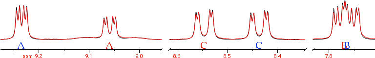 The visible effect of chemical exchange is the broadening of the lines. The effect is dramatic at the coalescence, when two of the corresponding signals of the exchanging species become one.
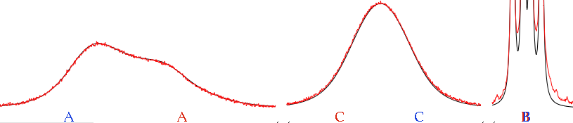 The temperature of coalescence depends on:
The direct consequence is that:
Look at the coalescence peak marked as CC. How can you extract two values of chemical shifts, 2 Js and one rate of exchange from that mountain? Well, you can't start from here. You start from the spectrum at a low temperature, where there's no exchange, and measure all the parameters but the exchange rate. Then, hopefully, it would be enough to introduce this rate to simulate the spectra at all the other temperatures. In practice, everything always changes, but slowly. At the slowest temperatures and at the highest ones, it is difficult to separate the effect of relaxation from that of exchange, because both contribute to a similar broadening. Near coalescence, the effect of the broadening caused by exchange is two orders of magnitude larger than the broadening caused by relaxation. In practice, even if the error in estimating relaxation is 100% of the value, the error in estimating exchange is only 1%, therefore more than acceptable. Far from coalescence, instead, you have to be cautious. The simplest thing to do is to verify that the T₂ changes monotonically with temperature.
In practice you collect 10 or more spectra at different temperatures. You also need the calibration curve of your probe (the instrument only reports the temperature around the probe; you need to know the temperature inside it, which can be measured spectroscopically, with a sample of methanol).
After extracting, by simulation, the rate of the exchange at each temperature, the plot of ln(k/T) versus 1/T gives a straight line; the enthalpy of activation can be derived from the slope and the entropy is derived from the intercept (Eyring equation). It's a mystery if these enthaply and entropy quantities remain the same at all temperatures or not. The linear plot should tell these things and will also tell if the whole work was correct or not.
If your software allows a computational least-square fit you can well try it, but I personally prefer the simple, old-style, manual fit. In theory there's no advantage in using a computational method, because the algorithm that finds the global minimum hasn't been invented yet. There is, however, something that a computer can do and we can't. It is the grand single fit of the whole experiment (the 10+ spectra) to find, via least squares, not the rates of exchange but directly the enthaply and entropy of activation. (They told me) the existence of this program has been mentioned in literature (years ago) but the program itself is not available.
The visible effect of chemical exchange is the broadening of the lines. The effect is dramatic at the coalescence, when two of the corresponding signals of the exchanging species become one.The temperature of coalescence depends on:- the exchange rate
- the difference in Hz
The direct consequence is that:
- a species with n signals can have up to n different temperatures of coalescence (in the pictures, n = 3)
- they change with the magnetic field
Look at the coalescence peak marked as CC. How can you extract two values of chemical shifts, 2 Js and one rate of exchange from that mountain? Well, you can't start from here. You start from the spectrum at a low temperature, where there's no exchange, and measure all the parameters but the exchange rate. Then, hopefully, it would be enough to introduce this rate to simulate the spectra at all the other temperatures. In practice, everything always changes, but slowly. At the slowest temperatures and at the highest ones, it is difficult to separate the effect of relaxation from that of exchange, because both contribute to a similar broadening. Near coalescence, the effect of the broadening caused by exchange is two orders of magnitude larger than the broadening caused by relaxation. In practice, even if the error in estimating relaxation is 100% of the value, the error in estimating exchange is only 1%, therefore more than acceptable. Far from coalescence, instead, you have to be cautious. The simplest thing to do is to verify that the T₂ changes monotonically with temperature.
In practice you collect 10 or more spectra at different temperatures. You also need the calibration curve of your probe (the instrument only reports the temperature around the probe; you need to know the temperature inside it, which can be measured spectroscopically, with a sample of methanol).
After extracting, by simulation, the rate of the exchange at each temperature, the plot of ln(k/T) versus 1/T gives a straight line; the enthalpy of activation can be derived from the slope and the entropy is derived from the intercept (Eyring equation). It's a mystery if these enthaply and entropy quantities remain the same at all temperatures or not. The linear plot should tell these things and will also tell if the whole work was correct or not.
If your software allows a computational least-square fit you can well try it, but I personally prefer the simple, old-style, manual fit. In theory there's no advantage in using a computational method, because the algorithm that finds the global minimum hasn't been invented yet. There is, however, something that a computer can do and we can't. It is the grand single fit of the whole experiment (the 10+ spectra) to find, via least squares, not the rates of exchange but directly the enthaply and entropy of activation. (They told me) the existence of this program has been mentioned in literature (years ago) but the program itself is not available.
Sunday, 13 July 2008
Relationships
A system of 3 different protons has 12 lines. The same system, made of ²H nuclei, has 27 lines. Both systems can be described with 3 shifts and 3 coupling constants. That's obvious. Add a common line-width: 7 parameters to describe 27 or 12 lines.
There are many other "obvious" relationships that often reduce the degree of freedom of the problem. The group CH₃-CH-CH₃ contains many more hydrogens, but is described by only 2 or 3 parameters (because of the magnetic equivalence). A para- (or ortho-) di-substituted benzene, if the substituent is the same, is symmetric: all parameters are duplicated. Tin is a mixture of isotopes, 3 of them are magnetically active. If you want to simulate the proton spectrum of a tin compound, you have to declare 3 or 4 systems, but their parameters (shifts, couplings), neglecting the isotope effects, are the same. The above 3 examples can be handled by the software. Summarizing:
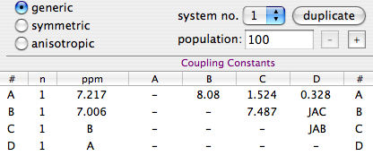 with the symmetry-aware equivalent:
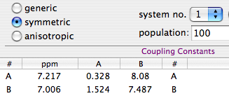 (pictures courtesy of www.inmr.net)
While it's important that the software directly implements the listed concepts, it's also useful that it understands additional relations defined directly by the user and specific for his/her problem. The first picture exemplifies the idea. The user renounced to the advantage of symmetry and the table of couplings is large. The number of parameters is still low, because he declared 4 relationships. For example, he declared that the shift of hydrogen C is the same as hydrogen B. This is the simplest form of relation (equality), that is implemented through symbolic parameters.
When are relations really useful? First example: transverse relaxation times. Quite often these simulation are performed assuming that all the nuclei have the same T₂ (same line-width). In a few cases, when one or two nuclei relax faster, you are forced to declare the individual widths. To keep the total number of parameters low, I prefer an intermediate solution: dividing the nuclei in two classes. There are only two parameters for the line-widths. This is possible if the software allows me to declare symbolic values. Excel allows me to fill a cell with numbers, text or expressions, at will, but doesn't understand NMR. I have cited Excel just to make the concept clear. The above picture shows that is possible to use symbols instead of numbers inside an NMR software.
Exploring the same web site you can see that symbolic values have been able to solve all sorts of problems:
There are many other "obvious" relationships that often reduce the degree of freedom of the problem. The group CH₃-CH-CH₃ contains many more hydrogens, but is described by only 2 or 3 parameters (because of the magnetic equivalence). A para- (or ortho-) di-substituted benzene, if the substituent is the same, is symmetric: all parameters are duplicated. Tin is a mixture of isotopes, 3 of them are magnetically active. If you want to simulate the proton spectrum of a tin compound, you have to declare 3 or 4 systems, but their parameters (shifts, couplings), neglecting the isotope effects, are the same. The above 3 examples can be handled by the software. Summarizing:
- magnetic equivalence
- symmetry
- isotopic mixture
with the symmetry-aware equivalent:(pictures courtesy of www.inmr.net)While it's important that the software directly implements the listed concepts, it's also useful that it understands additional relations defined directly by the user and specific for his/her problem. The first picture exemplifies the idea. The user renounced to the advantage of symmetry and the table of couplings is large. The number of parameters is still low, because he declared 4 relationships. For example, he declared that the shift of hydrogen C is the same as hydrogen B. This is the simplest form of relation (equality), that is implemented through symbolic parameters.
When are relations really useful? First example: transverse relaxation times. Quite often these simulation are performed assuming that all the nuclei have the same T₂ (same line-width). In a few cases, when one or two nuclei relax faster, you are forced to declare the individual widths. To keep the total number of parameters low, I prefer an intermediate solution: dividing the nuclei in two classes. There are only two parameters for the line-widths. This is possible if the software allows me to declare symbolic values. Excel allows me to fill a cell with numbers, text or expressions, at will, but doesn't understand NMR. I have cited Excel just to make the concept clear. The above picture shows that is possible to use symbols instead of numbers inside an NMR software.
Exploring the same web site you can see that symbolic values have been able to solve all sorts of problems:
Thursday, 10 July 2008
Checklist
Now that you know about the three main approaches, where to go from here?
If you want to use one of the methods for fitting a spin system (see yesterday's post), the simplest (and single) thing to do is to read the manual of your program. If it's too short, reading it will require a little investment of time. If it doesn't help, it either means that your program is extremely intuitive or that you need a different program. If, instead, the manual is very long, there are two cases: either the program is very powerful and well documented, so there's a lot of things to learn from it, or the program and its manual are a crappy mess.
There are a lot of advantages if the same program performs both processing and simulation; it means: less things to learn, a couple of export/import operations are avoided, there are more users (i.e. the program has been more tested), the interface is probably simplified (because they are general-purpose programs targeted at the casual user). The disadvantages (compared to a specialized program) may be a limited set of features.
It's also extremely convenient if the same program implements all the three fitting methods outlined yesterday AND dynamic NMR. This gives you the option to switch with no effort from any method to any other. If, instead, you use a different program for each method, and the first method you try turns out to be inappropriate, you have to redeclare the terms of your problem and re-import the experimental data... quite boring!
Comparing different programs
Not all programs are equal. Features to look for when comparing two of them:
- Can you adjust the parameters manually (graphically)?
- Are the plots (experimental and theoretical) overlapped?
- Can you define symmetry relations?
- How many systems can you define?
- Can you define relations between parameters of different systems?
- How many nuclei can you define?
- Can you define all kinds of spins?
- Are dipolar couplings handled?
- Is Dynamic NMR included?
- Is Total-Lineshape Fitting included?
- Is a LAOCOON-like Fitting included?
- Can you change the shape of the peaks or are they exclusively Lorentzian?
- Are the chemical shifts measured in ppm rather than in Hz?
- Can you declare a spin system by its ChemDraw formula?
- Once you have extracted the parameters, can you generate formatted lists of these parameters? How many formats?
- If your program includes a "multiplet analyzer", does it talk with the simulation module?
Wednesday, 9 July 2008
Arsenal
When you are able to process an NMR spectrum; when you are also able to simulate the same spectrum (starting from the definition of a spin system); then you are ready to fit the two, one against the other. People tend to skip all the intermediate stages. I would not. If I can't write the single words, I won't be able to write a sentence. Yesterday I said that the simulation of a spin system is a useful exercise to understand a few principles of NMR; now I need to stress that it's also a useful exercise before you move on to the extraction of the NMR parameters by simulation. Once you have the two main ingredients, the experimental spectrum and the synthetic one, there are three main methods to perform the fit; each one has a reason to exist.
(1) Manual Adjustment
This can work if the spectrum, or portions of it, can be interpreted with first-order rules. Chemical shifts are easy to fit manually, because it's enough to literally drag each multiplet in place. The coupling constants can be adjusted in order, from the most evident (large) one to the most difficult (small) to extract. The process is simplified when the experimental multiplets are well resolved; in other words: apply a Lorentz-to-Gauss resolution enhancement by weighting the FID. Manual adjustment has become quite popular after the advent of interactive applications in the 90s. Don't dismiss it as "naive": it is certainly more accurate than extracting the coupling constants directly from the list of frequencies (which is an accepted and widespread practice). Visual fitting can be difficult with second-order spectra, but not for a skilled operator. The trick of the experts is to monitor the position of the weak combination lines. They are forbidden transitions that appear as tiny satellites. If you can simulate them exactly, the rest comes naturally in place. They are diagnostic, like canaries in a coal mine.
(2) Laocoon
This was the name of the first popular program used to extract the Js from second-order, complicated multiplets. The program is no more in use today, but the method is still excellent. Quite simply it compares a list of experimental frequencies with a list of theoretical lines. Then improves the spectroscopic parameters according to the least squares principle. A lot of useful information is ignored, but this is also the strength of the method. When there is too much noise, or the baseline is problematic, or a solvent hides part of the spectrum, etc... you simply can't extract all the information from the spectrum, or you can but the intensities are not dependable. It's better to feed the algorithm with minimal selected data of high quality than hoping that a mass of errors can mutually compensate each other. With Laocoon it's not even necessary to match all the lines; as you can expect, the condition is that the number of parameters to guess must be less than the number of the lines. Despite the simplicity, this method requires more work, because you have to assign/match each experimental line to a theoretical line. This job looks trivial at the end of the process, because it's enough to match the lines in order of frequency. It's different when the starting guess is largely inaccurate. A single mismatch, in this case, is simple to discover, if you know the trick. The column of the residual errors will contain two large and opposite values. They correspond to the "swapped" lines. All considered, the most difficult part, for the user, is to read the manual of his/her program.
Here, more than in any other case, a Lorentz-to-Gauss weighting is beneficial: remember that you are not starting from the raw data points, but from the table of frequencies ("peak-picking"). It is well known that the position of the maxima of a doublet doesn't coincide with the true line frequencies, when peaks are broad.
 picture courtesy of the nmr-analysis blog.
(3) Total Line-shape (TLS)
I suspect that this approach derives, historically, from dynamic NMR, (the simulation of internal rotations, like in the case of DMF). You can, indeed, simulate a "static" system with a dynamic program, if the exchange rate is zero. DNMR (and the programs that follow the same principle) don't recalculate the single lines (frequencies, intensities) but other sets of parameters that are used, eventually, to create the synthetic spectrum (plot). The latter can be compared, point by point, to the experiment, and the least squares are calculated from the difference. This is a great simplification for the user, compared to LAOCOON, because it's no more necessary to assign the lines. An higher quality of the experimental spectrum is however required, because the program now also employs the intensity information, and this information must be correct. Therefore the baseline must be flat and no extraneous peak can be present (it is trivial, however, to artificially delete isolated extraneous peaks/humps). Summarizing: you must spend time on processing the experimental spectrum.
We have seen that the first two methods prefer gaussian line-shapes.
This is not necessary with TLS, but we have the inverse problem: if you have already prepared the experimental spectrum for the other kinds of fit (with Gaussian shapes), can you perform a total lineshape fit? The answer is "NO" if we look at the original formulation of the method, but in practice it is possible, with some commercial package, to work with both kinds of shapes (and anything in between too).
Don't be mislead by the name "Total": nobody fits the whole spectrum, but only portions of it. Most of the tricks we learned when fitting singlets (and collection of not-organized peaks) can be recycled with TLS. Actually, there is a minimal difference, from a mathematical point of view. In TLS, the algorithm varies a collection of parameters. They give a collection of lines, that are used to simulate the spectrum. In deconvolution, the algorithm directly start from the frequencies. That's the first difference. There is also a procedural difference: TLS has a built-in mechanism to escape from local minima. In practice, in the first stage of the fitting, a line broadening is applied that blurs the details. Once the multiplets has been set in the proper place, the broadening is removed and the details are taken into account. With plain line-fitting, there is no such need, because the first guess is extracted from the experimental spectrum itself, therefore everything is always in the right place (nearly).
If we called the previous method by the name of the first program implementing it, then TLS could be called, in a similar way, "DAVINS".
(1) Manual Adjustment
This can work if the spectrum, or portions of it, can be interpreted with first-order rules. Chemical shifts are easy to fit manually, because it's enough to literally drag each multiplet in place. The coupling constants can be adjusted in order, from the most evident (large) one to the most difficult (small) to extract. The process is simplified when the experimental multiplets are well resolved; in other words: apply a Lorentz-to-Gauss resolution enhancement by weighting the FID. Manual adjustment has become quite popular after the advent of interactive applications in the 90s. Don't dismiss it as "naive": it is certainly more accurate than extracting the coupling constants directly from the list of frequencies (which is an accepted and widespread practice). Visual fitting can be difficult with second-order spectra, but not for a skilled operator. The trick of the experts is to monitor the position of the weak combination lines. They are forbidden transitions that appear as tiny satellites. If you can simulate them exactly, the rest comes naturally in place. They are diagnostic, like canaries in a coal mine.
(2) Laocoon
This was the name of the first popular program used to extract the Js from second-order, complicated multiplets. The program is no more in use today, but the method is still excellent. Quite simply it compares a list of experimental frequencies with a list of theoretical lines. Then improves the spectroscopic parameters according to the least squares principle. A lot of useful information is ignored, but this is also the strength of the method. When there is too much noise, or the baseline is problematic, or a solvent hides part of the spectrum, etc... you simply can't extract all the information from the spectrum, or you can but the intensities are not dependable. It's better to feed the algorithm with minimal selected data of high quality than hoping that a mass of errors can mutually compensate each other. With Laocoon it's not even necessary to match all the lines; as you can expect, the condition is that the number of parameters to guess must be less than the number of the lines. Despite the simplicity, this method requires more work, because you have to assign/match each experimental line to a theoretical line. This job looks trivial at the end of the process, because it's enough to match the lines in order of frequency. It's different when the starting guess is largely inaccurate. A single mismatch, in this case, is simple to discover, if you know the trick. The column of the residual errors will contain two large and opposite values. They correspond to the "swapped" lines. All considered, the most difficult part, for the user, is to read the manual of his/her program.
Here, more than in any other case, a Lorentz-to-Gauss weighting is beneficial: remember that you are not starting from the raw data points, but from the table of frequencies ("peak-picking"). It is well known that the position of the maxima of a doublet doesn't coincide with the true line frequencies, when peaks are broad.
picture courtesy of the nmr-analysis blog.(3) Total Line-shape (TLS)
I suspect that this approach derives, historically, from dynamic NMR, (the simulation of internal rotations, like in the case of DMF). You can, indeed, simulate a "static" system with a dynamic program, if the exchange rate is zero. DNMR (and the programs that follow the same principle) don't recalculate the single lines (frequencies, intensities) but other sets of parameters that are used, eventually, to create the synthetic spectrum (plot). The latter can be compared, point by point, to the experiment, and the least squares are calculated from the difference. This is a great simplification for the user, compared to LAOCOON, because it's no more necessary to assign the lines. An higher quality of the experimental spectrum is however required, because the program now also employs the intensity information, and this information must be correct. Therefore the baseline must be flat and no extraneous peak can be present (it is trivial, however, to artificially delete isolated extraneous peaks/humps). Summarizing: you must spend time on processing the experimental spectrum.
We have seen that the first two methods prefer gaussian line-shapes.
This is not necessary with TLS, but we have the inverse problem: if you have already prepared the experimental spectrum for the other kinds of fit (with Gaussian shapes), can you perform a total lineshape fit? The answer is "NO" if we look at the original formulation of the method, but in practice it is possible, with some commercial package, to work with both kinds of shapes (and anything in between too).
Don't be mislead by the name "Total": nobody fits the whole spectrum, but only portions of it. Most of the tricks we learned when fitting singlets (and collection of not-organized peaks) can be recycled with TLS. Actually, there is a minimal difference, from a mathematical point of view. In TLS, the algorithm varies a collection of parameters. They give a collection of lines, that are used to simulate the spectrum. In deconvolution, the algorithm directly start from the frequencies. That's the first difference. There is also a procedural difference: TLS has a built-in mechanism to escape from local minima. In practice, in the first stage of the fitting, a line broadening is applied that blurs the details. Once the multiplets has been set in the proper place, the broadening is removed and the details are taken into account. With plain line-fitting, there is no such need, because the first guess is extracted from the experimental spectrum itself, therefore everything is always in the right place (nearly).
If we called the previous method by the name of the first program implementing it, then TLS could be called, in a similar way, "DAVINS".
Tuesday, 8 July 2008
Spin Systems
A fortnight ago we saw how to fit a spectrum with a collection of curves. A more evolute approach is to fit the spectrum with a collection of NMR parameters (shifts and Js in the first place). There are two reasons to prefer the latter approach:
We have arrived to a large topic from an unusual path. We are in the field of quantum mechanic. It's easy in theory and, in practice, when the nuclei are few. When the number of nuclei in a spin system grows, no computer is fast enough to calculate precisely what happens. Somebody has also proposed to invert the roles, and create a super-computer with a large enough spin system (the quantum computer). That's even more difficult (try building a real molecule with 20 different nuclides!). When the number of nuclei is limited (e.g.: 10 protons), there is however no problem, at least with the older programs that diagonalize the Hamiltonian. I dedicated a post to the modern programs that can follow the evolution of a system under all kinds of effects. They have more calculations to do, are limited to smaller systems and, as it appeared from my old post, are oriented towards solid-state NMR.
Older programs are more popular in liquid-state NMR. I have already cited the free gNMR and SpiWorks. I have probably never cited Perch LE and Wind-NMR. Thay are all free (for academic users at least) and they all require Windows. Can you suggest a free solution for Linux and Mac users?
 It's not a surprise that, which such an abundance of free solutions, the commercial applications, in this present moment, are ignoring the field. The race now is at predicting the spectrum directly from the chemical structure. That's the third level. At the first level we have the frequencies and intensities of the single lines. At the second level we have shifts and couplings. At the third level we have the structure. If you only have the third level, you can verify your spectrum against the prediction, but if you want to publish your data you need to extract the Js directly from the experimental data. You can't do that without the second level, unless you are glad to standardize all your reports into lists of unspecified multiplets, like:
7.24, m (2H); 4.14, m (2H), 2.36, m (8H).....
The simulation of spin systems is also becoming a popular exercise for chemistry students new to the world of NMR. It's amazing how fast the magnetic field can change, even by orders of magnitude. After a while the game becomes repetitive, but it remains highly instructive for newcomers. An excellent starting point is an article by Carlos on the NMR Analysis Blog. It should be, however, complemented by practice, more than by further references. There is a minimal library of ready examples for Mac users. It contains the classic cases (orto-di-chloro-benzene, DMF), plus templates for small and medium-sized systems of 1/2 nuclei. In the case of DMF you can change not only the magnetic field, but also the temperature.
I don't want to bother you with theory, but one thing at least must be said: geminal couplings usually have a negative constant!
One more thing on practice too: Carlos said that not all NMR signals are symmetric. Personally I still believe into the myth that they are symmetric, like the human body. To be precise, neither are symmetric, but in practice this precision is useless and misleading. I rely on the IDEA of symmetry to recognize a friendly face and I rely on the IDEA of symmetry to recognize NMR signals. By the way: they too are friendly!
- you introduce logical restrictions into the model, for example you specify that the components of a triplet are in the ratio 1:2:1
- you overcome the job of measuring shifts and Js from line positions
We have arrived to a large topic from an unusual path. We are in the field of quantum mechanic. It's easy in theory and, in practice, when the nuclei are few. When the number of nuclei in a spin system grows, no computer is fast enough to calculate precisely what happens. Somebody has also proposed to invert the roles, and create a super-computer with a large enough spin system (the quantum computer). That's even more difficult (try building a real molecule with 20 different nuclides!). When the number of nuclei is limited (e.g.: 10 protons), there is however no problem, at least with the older programs that diagonalize the Hamiltonian. I dedicated a post to the modern programs that can follow the evolution of a system under all kinds of effects. They have more calculations to do, are limited to smaller systems and, as it appeared from my old post, are oriented towards solid-state NMR.
Older programs are more popular in liquid-state NMR. I have already cited the free gNMR and SpiWorks. I have probably never cited Perch LE and Wind-NMR. Thay are all free (for academic users at least) and they all require Windows. Can you suggest a free solution for Linux and Mac users?
It's not a surprise that, which such an abundance of free solutions, the commercial applications, in this present moment, are ignoring the field. The race now is at predicting the spectrum directly from the chemical structure. That's the third level. At the first level we have the frequencies and intensities of the single lines. At the second level we have shifts and couplings. At the third level we have the structure. If you only have the third level, you can verify your spectrum against the prediction, but if you want to publish your data you need to extract the Js directly from the experimental data. You can't do that without the second level, unless you are glad to standardize all your reports into lists of unspecified multiplets, like:7.24, m (2H); 4.14, m (2H), 2.36, m (8H).....
The simulation of spin systems is also becoming a popular exercise for chemistry students new to the world of NMR. It's amazing how fast the magnetic field can change, even by orders of magnitude. After a while the game becomes repetitive, but it remains highly instructive for newcomers. An excellent starting point is an article by Carlos on the NMR Analysis Blog. It should be, however, complemented by practice, more than by further references. There is a minimal library of ready examples for Mac users. It contains the classic cases (orto-di-chloro-benzene, DMF), plus templates for small and medium-sized systems of 1/2 nuclei. In the case of DMF you can change not only the magnetic field, but also the temperature.
I don't want to bother you with theory, but one thing at least must be said: geminal couplings usually have a negative constant!
One more thing on practice too: Carlos said that not all NMR signals are symmetric. Personally I still believe into the myth that they are symmetric, like the human body. To be precise, neither are symmetric, but in practice this precision is useless and misleading. I rely on the IDEA of symmetry to recognize a friendly face and I rely on the IDEA of symmetry to recognize NMR signals. By the way: they too are friendly!
Monday, 7 July 2008
Fixed Focus
All cameras need to be focused before shooting. There are 3 alternatives: manual focus, autofocus and fixed focus. The latter is an economical choice that can't work under all circumstances, it's OK only when the depth of field is large enough. This depth depends on the characteristics of the lens.
I can see a similarity in NMR spectroscopy. The phase correction of an high-resolution spectrum is like a lens with a limited depth of field (think to a telescope, if you are more familiar with them; the telescope is an example of a lens with a narrow depth of field). Starting from the optimal correction, a minimal change in the phase correction parameter (movement of the lens, in the parallel example) causes a visible negative effect on the spectrum (clearness of the image). It's not enough to copy the phase correction from a spectrum to the other, you must use either manual or automatic correction or both. Like it or not, you'll become an expert in the field.
Weighting is much more tolerant to a small change of the parameters, to the point that most of us use the "Fixed Focus" approach. We can even store the optimal value inside our standard parameters and forget about it. When you have forgotten it, it's arduous to improve your skill; DSP (digital signal processing) contains too much theory and practice is time consuming.
My rules are:
While I usually recommend to observe and practice, because 50% of NMR can be deducted with common sense, there is a case where you need the theory, otherwise you go nowhere. If you keep weighting a standard COSY spectrum with the same functions that you use in 1D spectroscopy, you'll always get star-shaped peaks like this:
 [after exponential weighting along both dimensions]
It's only theory that tells you that a symmetric FID corresponds to a symmetric spectrum, therefore if your weighted FID has a symmetric envelope, the dispersion component will be attenuated in frequency domain. In simpler words: use a sine-bell. It's counter-intuitive to zero the less noisy part of your spectrum, but look at the final effect:
 [after weighting with two pure sine bells]
I can see a similarity in NMR spectroscopy. The phase correction of an high-resolution spectrum is like a lens with a limited depth of field (think to a telescope, if you are more familiar with them; the telescope is an example of a lens with a narrow depth of field). Starting from the optimal correction, a minimal change in the phase correction parameter (movement of the lens, in the parallel example) causes a visible negative effect on the spectrum (clearness of the image). It's not enough to copy the phase correction from a spectrum to the other, you must use either manual or automatic correction or both. Like it or not, you'll become an expert in the field.
Weighting is much more tolerant to a small change of the parameters, to the point that most of us use the "Fixed Focus" approach. We can even store the optimal value inside our standard parameters and forget about it. When you have forgotten it, it's arduous to improve your skill; DSP (digital signal processing) contains too much theory and practice is time consuming.
My rules are:
- Weighting is an alteration of the spectrum. An altered spectrum may look ugly, don't worry.
- It's more important to know what I want to obtain (where I want to go) that the way to go there, because many roads lead to the same place, but I must be able to recognize my destination if I arrive there.
While I usually recommend to observe and practice, because 50% of NMR can be deducted with common sense, there is a case where you need the theory, otherwise you go nowhere. If you keep weighting a standard COSY spectrum with the same functions that you use in 1D spectroscopy, you'll always get star-shaped peaks like this:
 [after exponential weighting along both dimensions]
It's only theory that tells you that a symmetric FID corresponds to a symmetric spectrum, therefore if your weighted FID has a symmetric envelope, the dispersion component will be attenuated in frequency domain. In simpler words: use a sine-bell. It's counter-intuitive to zero the less noisy part of your spectrum, but look at the final effect:
 [after weighting with two pure sine bells]
Subscribe to:
Posts (Atom)